

Does The Nec/oesc Require A Temporary Service To Have A Meter?
Measurements and Fault Analysis
"It is improve to exist roughly correct than precisely wrong." — Alan Greenspan
The Doubtfulness of Measurements
Some numerical statements are exact: Mary has iii brothers, and 2 + two = four. Still, all measurements accept some caste of uncertainty that may come up from a multifariousness of sources. The process of evaluating the dubiousness associated with a measurement consequence is often chosen doubtfulness analysis or fault analysis. The complete argument of a measured value should include an estimate of the level of conviction associated with the value. Properly reporting an experimental result forth with its incertitude allows other people to brand judgments about the quality of the experiment, and it facilitates meaningful comparisons with other similar values or a theoretical prediction. Without an incertitude estimate, information technology is impossible to answer the bones scientific question: "Does my outcome concur with a theoretical prediction or results from other experiments?" This question is fundamental for deciding if a scientific hypothesis is confirmed or refuted. When we make a measurement, we generally assume that some verbal or truthful value exists based on how we define what is being measured. While we may never know this truthful value exactly, we endeavour to find this platonic quantity to the best of our ability with the fourth dimension and resources available. As nosotros make measurements by unlike methods, or fifty-fifty when making multiple measurements using the same method, we may obtain slightly unlike results. So how exercise we report our findings for our best approximate of this elusive true value? The most mutual manner to show the range of values that nosotros believe includes the true value is:
( i )
measurement = (all-time judge ± uncertainty) units
Allow's take an example. Suppose you want to discover the mass of a gold ring that you would like to sell to a friend. You do not want to jeopardize your friendship, so you want to go an accurate mass of the ring in order to charge a fair market price. You gauge the mass to be between 10 and 20 grams from how heavy it feels in your hand, but this is not a very precise judge. Afterward some searching, you find an electronic residual that gives a mass reading of 17.43 grams. While this measurement is much more than precise than the original judge, how do you know that it is accurate, and how confident are you that this measurement represents the true value of the ring'southward mass? Since the digital brandish of the balance is express to 2 decimal places, you could study the mass as k = 17.43 ± 0.01 1000. 17.44 ± 0.02 g. Accurateness is the closeness of agreement betwixt a measured value and a true or accepted value. Measurement mistake is the amount of inaccuracy. Precision is a measure out of how well a upshot can be adamant (without reference to a theoretical or true value). It is the degree of consistency and understanding among independent measurements of the same quantity; also the reliability or reproducibility of the result. The incertitude estimate associated with a measurement should account for both the accuracy and precision of the measurement.
( two )
Relative Incertitude = 
dubiousness measured quantity
Instance: m = 75.5 ± 0.v grand = 0.006 = 0.vii%.
( 3 )
Relative Error =
measured value − expected value expected value
If the expected value for m is 80.0 g, and so the relative error is: = −0.056 = −5.6% Note: The minus sign indicates that the measured value is less than the expected value.
Types of Errors
Measurement errors may be classified as either random or systematic, depending on how the measurement was obtained (an musical instrument could cause a random fault in one situation and a systematic error in another).
Random errors are statistical fluctuations (in either direction) in the measured data due to the precision limitations of the measurement device. Random errors can exist evaluated through statistical analysis and tin can exist reduced by averaging over a big number of observations (see standard fault).
Systematic errors are reproducible inaccuracies that are consistently in the same direction. These errors are hard to discover and cannot be analyzed statistically. If a systematic error is identified when calibrating confronting a standard, applying a correction or correction factor to recoup for the consequence can reduce the bias. Unlike random errors, systematic errors cannot exist detected or reduced past increasing the number of observations.
When making careful measurements, our goal is to reduce as many sources of error as possible and to keep track of those errors that we can non eliminate. Information technology is useful to know the types of errors that may occur, so that nosotros may recognize them when they arise. Common sources of mistake in physics laboratory experiments:
Incomplete definition (may be systematic or random) — One reason that it is incommunicable to brand verbal measurements is that the measurement is non e'er conspicuously defined. For example, if two different people measure the length of the same cord, they would probably become different results considering each person may stretch the string with a different tension. The best way to minimize definition errors is to carefully consider and specify the atmospheric condition that could affect the measurement. Failure to business relationship for a factor (usually systematic) — The most challenging office of designing an experiment is trying to command or account for all possible factors except the one contained variable that is being analyzed. For example, you lot may inadvertently ignore air resistance when measuring free-autumn acceleration, or you may neglect to account for the upshot of the Earth'southward magnetic field when measuring the field about a small magnet. The best manner to account for these sources of error is to brainstorm with your peers about all the factors that could possibly affect your result. This brainstorm should be washed before beginning the experiment in order to plan and account for the misreckoning factors before taking data. Sometimes a correction tin can be applied to a effect after taking data to account for an error that was not detected earlier. Environmental factors (systematic or random) — Be aware of errors introduced past your immediate working environment. You may need to take account for or protect your experiment from vibrations, drafts, changes in temperature, and electronic dissonance or other furnishings from nearby apparatus. Instrument resolution (random) — All instruments accept finite precision that limits the power to resolve small measurement differences. For case, a meter stick cannot be used to distinguish distances to a precision much better than about half of its smallest calibration division (0.5 mm in this case). One of the best means to obtain more precise measurements is to employ a null difference method instead of measuring a quantity direct. Null or balance methods involve using instrumentation to measure out the difference betwixt two like quantities, one of which is known very accurately and is adjustable. The adaptable reference quantity is varied until the difference is reduced to nil. The two quantities are and then balanced and the magnitude of the unknown quantity tin can be found by comparison with a measurement standard. With this method, problems of source instability are eliminated, and the measuring instrument can be very sensitive and does not fifty-fifty demand a scale. Calibration (systematic) — Whenever possible, the calibration of an instrument should be checked earlier taking data. If a calibration standard is not bachelor, the accuracy of the musical instrument should be checked by comparing with another instrument that is at to the lowest degree as precise, or by consulting the technical information provided by the manufacturer. Calibration errors are usually linear (measured every bit a fraction of the full calibration reading), then that larger values consequence in greater accented errors. Zero offset (systematic) — When making a measurement with a micrometer caliper, electronic residuum, or electrical meter, e'er check the nothing reading get-go. Re-goose egg the instrument if possible, or at least measure out and tape the null offset so that readings can be corrected later. It is as well a expert idea to bank check the zilch reading throughout the experiment. Failure to null a device volition upshot in a abiding error that is more significant for smaller measured values than for larger ones. Concrete variations (random) — Information technology is always wise to obtain multiple measurements over the widest range possible. Doing so often reveals variations that might otherwise go undetected. These variations may phone call for closer examination, or they may be combined to find an boilerplate value. Parallax (systematic or random) — This mistake can occur whenever at that place is some distance betwixt the measuring scale and the indicator used to obtain a measurement. If the observer's eye is not squarely aligned with the pointer and scale, the reading may be besides high or low (some analog meters have mirrors to help with this alignment). Instrument drift (systematic) — Most electronic instruments have readings that drift over time. The amount of drift is generally not a concern, just occasionally this source of error can be significant. Lag time and hysteresis (systematic) — Some measuring devices require time to reach equilibrium, and taking a measurement earlier the instrument is stable volition result in a measurement that is too high or low. A common example is taking temperature readings with a thermometer that has not reached thermal equilibrium with its environment. A similar result is hysteresis where the instrument readings lag behind and appear to accept a "retentivity" issue, as data are taken sequentially moving up or down through a range of values. Hysteresis is most ordinarily associated with materials that become magnetized when a irresolute magnetic field is applied. Personal errors come from carelessness, poor technique, or bias on the part of the experimenter. The experimenter may measure out incorrectly, or may employ poor technique in taking a measurement, or may introduce a bias into measurements by expecting (and inadvertently forcing) the results to concord with the expected outcome.
Gross personal errors, sometimes called mistakes or blunders, should be avoided and corrected if discovered. As a rule, personal errors are excluded from the error assay discussion because it is by and large assumed that the experimental result was obtained past post-obit right procedures. The term man error should also exist avoided in error assay discussions because it is too full general to be useful.
Estimating Experimental Uncertainty for a Single Measurement
Any measurement yous make will accept some dubiety associated with information technology, no matter the precision of your measuring tool. So how do y'all determine and report this incertitude?
The uncertainty of a unmarried measurement is express by the precision and accuracy of the measuring instrument, forth with any other factors that might affect the ability of the experimenter to make the measurement.
For example, if you are trying to employ a meter stick to measure out the bore of a tennis ball, the dubiousness might be ± 5 mm, ± two mm.
( iv )
Measurement = (measured value ± standard dubiety) unit of measurement of measurement
where the ± standard uncertainty indicates approximately a 68% confidence interval (see sections on Standard Deviation and Reporting Uncertainties). 6.seven ± 0.2 cm.
Example: Diameter of tennis ball =
Estimating Uncertainty in Repeated Measurements
Suppose you time the period of oscillation of a pendulum using a digital instrument (that you assume is measuring accurately) and find: T = 0.44 seconds. This single measurement of the catamenia suggests a precision of ±0.005 s, but this instrument precision may not give a complete sense of the doubtfulness. If you lot repeat the measurement several times and examine the variation amidst the measured values, y'all can get a improve idea of the dubiousness in the menstruation. For example, here are the results of v measurements, in seconds: 0.46, 0.44, 0.45, 0.44, 0.41.
( 5 )
Average (mean) =
x ane + x two + 
Northward
For this state of affairs, the best estimate of the menstruation is the average, or mean.
Whenever possible, repeat a measurement several times and boilerplate the results. This average is mostly the best estimate of the "true" value (unless the data set is skewed by one or more outliers which should be examined to determine if they are bad data points that should be omitted from the average or valid measurements that require further investigation). Generally, the more repetitions yous make of a measurement, the better this estimate will exist, but exist conscientious to avoid wasting time taking more measurements than is necessary for the precision required.
Consider, equally some other example, the measurement of the width of a slice of paper using a meter stick. Being careful to proceed the meter stick parallel to the edge of the paper (to avert a systematic error which would cause the measured value to be consistently higher than the correct value), the width of the paper is measured at a number of points on the sheet, and the values obtained are entered in a data table. Note that the terminal digit is only a rough estimate, since it is difficult to read a meter stick to the nearest tenth of a millimeter (0.01 cm). 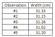
( 6 )
Average =
= = 31.19 cm sum of observed widths no. of observations
This average is the best available estimate of the width of the piece of paper, but it is certainly non exact. We would have to average an infinite number of measurements to approach the truthful mean value, and even and then, nosotros are non guaranteed that the mean value is authentic considering there is yet some systematic mistake from the measuring tool, which can never be calibrated perfectly. So how practice we express the uncertainty in our average value? One way to express the variation amongst the measurements is to use the average deviation. This statistic tells us on average (with fifty% conviction) how much the individual measurements vary from the mean.
( 7 )
d =
|x 1 − x | + |10 ii − x | + N
Notwithstanding, the standard difference is the most common manner to characterize the spread of a data set. The standard deviation is e'er slightly greater than the average divergence, and is used because of its association with the normal distribution that is frequently encountered in statistical analyses.
Standard Deviation
To calculate the standard divergence for a sample of N measurements:
-
i
Sum all the measurements and separate past Northward to get the average, or mean. -
ii
At present, decrease this average from each of the Northward measurements to obtain Due north "deviations". -
3
Square each of these N deviations and add them all upwardly. -
iv
Divide this result by( N − 1)
and take the square root.
We tin can write out the formula for the standard deviation as follows. Allow the North measurements be called x one, 10 ii, ..., 10N . Let the average of the N values be called x . δ x i = ten i − 10 , for i = i, two,
In our previous instance, the average width x d = 0.086 cm. s = x ± ii s,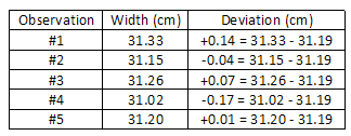 The boilerplate divergence is:
= 0.12 cm. 
(0.14)2 + (0.04)2 + (0.07)2 + (0.17)ii + (0.01)2 5 − 1
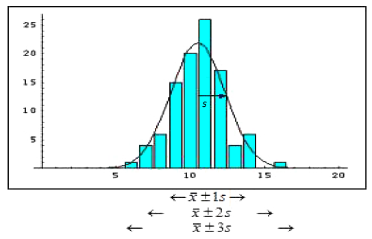
Figure 1
Standard Divergence of the Mean (Standard Mistake)
When we report the boilerplate value of N measurements, the incertitude nosotros should associate with this average value is the standard departure of the mean, often called the standard error (SE).
( 9 )
σ x =
due south

N
The standard fault is smaller than the standard deviation by a factor of 1/ Boilerplate paper width = 31.19 ± 0.05 cm.
. N
. 5
Anomalous Information
The first step you should take in analyzing data (and even while taking data) is to examine the data set as a whole to look for patterns and outliers. Anomalous data points that prevarication outside the general trend of the data may suggest an interesting phenomenon that could lead to a new discovery, or they may simply be the result of a mistake or random fluctuations. In whatsoever case, an outlier requires closer test to determine the cause of the unexpected result. Extreme information should never be "thrown out" without clear justification and explanation, because you may be discarding the most meaning function of the investigation! However, if you lot tin can clearly justify omitting an inconsistent information point, then you should exclude the outlier from your assay so that the average value is non skewed from the "true" hateful.
Partial Doubtfulness Revisited
When a reported value is determined past taking the average of a set up of independent readings, the partial uncertainty is given by the ratio of the dubiousness divided by the average value. For this example,
( 10 )
Partial doubt = = = 0.0016 ≈ 0.two%
Annotation that the fractional dubiousness is dimensionless but is often reported as a percentage or in parts per million (ppm) to emphasize the fractional nature of the value. A scientist might also make the statement that this measurement "is expert to about 1 part in 500" or "precise to near 0.two%". The fractional dubiousness is also important considering it is used in propagating uncertainty in calculations using the issue of a measurement, equally discussed in the next department.
Propagation of Uncertainty
Suppose we want to make up one's mind a quantity f, which depends on 10 and maybe several other variables y, z, etc. We want to know the error in f if we measure x, y, ... with errors σ 10 , σ y , ... Examples:
( 11 )
f = xy (Area of a rectangle)
( 12 )
f = p cos θ ( x -component of momentum)
( 13 )
f = x / t (velocity)
For a single-variable function f(x), the deviation in f can be related to the deviation in x using calculus:
( 14 )
δ f = 

Thus, taking the square and the average:
( fifteen )
δ f 2 =
δ x 2 2
and using the definition of σ , nosotros become:
( 16 )
σ f = 
Examples: (a) f =
ten
( 17 )
=
1 2
x
( eighteen )
σ f =
, or = σ x 2
ten
(b) f = x 2
(c) f = cos θ
( 22 )
σ f = |sin θ | σ θ , or = |tan θ | σ θ Notation : in this situation, σ θ must be in radians.
In the case where f depends on two or more variables, the derivation above tin can exist repeated with minor modification. For ii variables, f(x, y), we have:
The partial derivative means differentiating f with respect to x holding the other variables fixed. Taking the square and the average, nosotros become the police force of propagation of uncertainty:
If the measurements of x and y are uncorrelated, then δ x δ y = 0,
Examples: (a) f = x + y
( 27 )
∴ σ f =
σ x two + σ y 2
When adding (or subtracting) independent measurements, the absolute uncertainty of the sum (or divergence) is the root sum of squares (RSS) of the individual accented uncertainties. When adding correlated measurements, the doubt in the consequence is merely the sum of the absolute uncertainties, which is always a larger doubtfulness gauge than adding in quadrature (RSS). Adding or subtracting a constant does not change the absolute uncertainty of the calculated value every bit long as the constant is an verbal value.
(b) f = xy
( 29 )
∴ σ f =

y 2 σ x 2 + ten 2 σ y 2
Dividing the previous equation by f = xy, nosotros get:
(c) f = 10 / y
Dividing the previous equation past f = 10 / y ,
When multiplying (or dividing) contained measurements, the relative uncertainty of the product (quotient) is the RSS of the individual relative uncertainties. When multiplying correlated measurements, the uncertainty in the consequence is just the sum of the relative uncertainties, which is e'er a larger uncertainty judge than adding in quadrature (RSS). Multiplying or dividing by a constant does not change the relative incertitude of the calculated value.
Annotation that the relative dubiety in f, equally shown in (b) and (c) above, has the same class for multiplication and sectionalization: the relative uncertainty in a product or quotient depends on the relative dubiousness of each individual term. Instance: Find uncertainty in five, where v = at
( 34 )
= = =
= 0.031 or three.1% 
(0.010)2 + (0.029)2
Notice that the relative uncertainty in t (ii.9%) is significantly greater than the relative doubtfulness for a (ane.0%), and therefore the relative doubt in v is essentially the same as for t (virtually 3%). Graphically, the RSS is like the Pythagorean theorem:
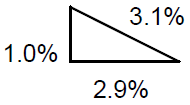
Figure 2
The total uncertainty is the length of the hypotenuse of a correct triangle with legs the length of each uncertainty component.
Timesaving approximation: "A chain is simply every bit strong equally its weakest link."
If i of the uncertainty terms is more than 3 times greater than the other terms, the root-squares formula tin be skipped, and the combined uncertainty is simply the largest incertitude. This shortcut tin can save a lot of time without losing whatsoever accuracy in the gauge of the overall uncertainty.
The Upper-Lower Bound Method of Incertitude Propagation
An alternative, and sometimes simpler process, to the wearisome propagation of uncertainty law is the upper-lower bound method of incertitude propagation. This alternative method does not yield a standard dubiety estimate (with a 68% confidence interval), but it does requite a reasonable estimate of the uncertainty for practically whatsoever situation. The basic thought of this method is to apply the uncertainty ranges of each variable to calculate the maximum and minimum values of the part. Yous tin also think of this procedure every bit examining the best and worst case scenarios. For example, suppose you measure an bending to be: θ = 25° ± 1° and you needed to find f = cos θ , then:
( 35 )
f max = cos(26°) = 0.8988
( 36 )
f min = cos(24°) = 0.9135
( 37 )
∴ f = 0.906 ± 0.007 

Note that even though θ was only measured to two significant figures, f is known to 3 figures. By using the propagation of uncertainty law: σ f = |sin θ | σ θ = (0.423)( π /180) = 0.0074
The uncertainty estimate from the upper-lower bound method is by and large larger than the standard dubiousness estimate establish from the propagation of incertitude constabulary, but both methods will give a reasonable estimate of the uncertainty in a calculated value.
The upper-lower jump method is especially useful when the functional relationship is not clear or is incomplete. One applied application is forecasting the expected range in an expense upkeep. In this case, some expenses may exist stock-still, while others may be uncertain, and the range of these uncertain terms could exist used to predict the upper and lower bounds on the total expense.
Meaning Figures
The number of significant figures in a value tin can be defined every bit all the digits between and including the first non-zero digit from the left, through the concluding digit. For instance, 0.44 has two significant figures, and the number 66.770 has v significant figures. Zeroes are significant except when used to locate the decimal indicate, as in the number 0.00030, which has 2 significant figures. Zeroes may or may not be significant for numbers like 1200, where information technology is not clear whether 2, three, or four meaning figures are indicated. To avoid this ambiguity, such numbers should exist expressed in scientific annotation to (e.thou. 1.20 × tenthree clearly indicates iii significant figures). When using a calculator, the display volition often prove many digits, merely some of which are meaningful (pregnant in a dissimilar sense). For case, if you lot desire to guess the area of a round playing field, yous might step off the radius to be 9 meters and utilize the formula: A = π r 2. When you lot compute this area, the figurer might study a value of 254.4690049 1000two. It would be extremely misleading to report this number equally the area of the field, considering it would suggest that you know the area to an absurd caste of precision—to within a fraction of a square millimeter! Since the radius is just known to i significant effigy, the terminal answer should too contain only one significant figure: Surface area = 3 × ten2 m2. From this example, we can encounter that the number of meaning figures reported for a value implies a certain degree of precision. In fact, the number of significant figures suggests a rough estimate of the relative dubiousness: The number of significant figures implies an judge relative dubiety:
i significant figure suggests a relative dubiety of about 10% to 100%
two meaning figures suggest a relative uncertainty of nigh 1% to x%
3 significant figures suggest a relative incertitude of nearly 0.1% to 1%
Utilise of Significant Figures for Unproblematic Propagation of Uncertainty
By post-obit a few uncomplicated rules, significant figures can be used to find the appropriate precision for a calculated result for the four virtually basic math functions, all without the use of complicated formulas for propagating uncertainties.
For multiplication and division, the number of significant figures that are reliably known in a product or quotient is the aforementioned as the smallest number of significant figures in whatever of the original numbers.
Example:
6.6 × 7328.7 48369.42 = 48 × 103
(2 meaning figures) (5 significant figures) (ii significant figures)
For addition and subtraction, the result should be rounded off to the last decimal place reported for the to the lowest degree precise number.
Examples:
223.64 5560.five + 54 + 0.008 278 5560.5
Uncertainty, Significant Figures, and Rounding
For the aforementioned reason that it is dishonest to study a result with more pregnant figures than are reliably known, the dubiousness value should also not exist reported with excessive precision. For example, information technology would be unreasonable for a student to report a result like:
( 38 )
measured density = 8.93 ± 0.475328 one thousand/cm3 Wrong!
The doubt in the measurement cannot possibly be known so precisely! In virtually experimental work, the confidence in the dubiety approximate is non much better than about ±50% considering of all the various sources of error, none of which can be known exactly. Therefore, uncertainty values should be stated to only 1 significant effigy (or peradventure ii sig. figs. if the first digit is a 1). Because experimental uncertainties are inherently imprecise, they should exist rounded to one, or at virtually 2, meaning figures. = measured density = eight.9 ± 0.v g/cmthree.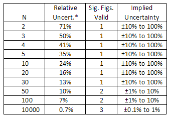 *The relative uncertainty is given by the estimate formula:
1
2(North − i)
An experimental value should be rounded to exist consistent with the magnitude of its doubt. This by and large means that the final significant figure in any reported value should exist in the same decimal identify every bit the uncertainty.
In most instances, this practice of rounding an experimental result to be consistent with the uncertainty approximate gives the same number of meaning figures as the rules discussed earlier for simple propagation of uncertainties for calculation, subtracting, multiplying, and dividing.
Caution: When conducting an experiment, it is important to keep in mind that precision is expensive (both in terms of time and textile resources). Practice not waste product your fourth dimension trying to obtain a precise result when merely a rough estimate is required. The cost increases exponentially with the amount of precision required, and so the potential benefit of this precision must exist weighed against the actress cost.
Combining and Reporting Uncertainties
In 1993, the International Standards Organization (ISO) published the first official worldwide Guide to the Expression of Uncertainty in Measurement. Before this time, doubtfulness estimates were evaluated and reported according to unlike conventions depending on the context of the measurement or the scientific subject. Here are a few key points from this 100-page guide, which tin can exist found in modified form on the NIST website. When reporting a measurement, the measured value should be reported forth with an estimate of the total combined standard incertitude U c
Conclusion: "When practise measurements agree with each other?"
We now accept the resources to respond the fundamental scientific question that was asked at the beginning of this mistake assay word: "Does my result hold with a theoretical prediction or results from other experiments?" By and large speaking, a measured upshot agrees with a theoretical prediction if the prediction lies inside the range of experimental uncertainty. Similarly, if 2 measured values have standard uncertainty ranges that overlap, then the measurements are said to be consistent (they agree). If the dubiousness ranges do not overlap, then the measurements are said to exist discrepant (they do not hold). Yet, you should recognize that these overlap criteria can requite two opposite answers depending on the evaluation and conviction level of the dubiousness. Information technology would exist unethical to arbitrarily inflate the doubt range only to make a measurement agree with an expected value. A better procedure would exist to discuss the size of the difference between the measured and expected values within the context of the doubtfulness, and try to discover the source of the discrepancy if the difference is truly significant. To examine your own data, you are encouraged to use the Measurement Comparison tool bachelor on the lab website. Here are some examples using this graphical analysis tool:
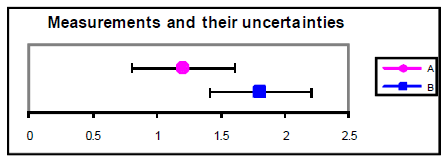
Figure 3
A = 1.2 ± 0.4 B = one.8 ± 0.4
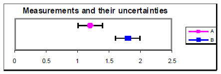
Figure four
An alternative method for determining understanding between values is to calculate the difference betwixt the values divided by their combined standard uncertainty. This ratio gives the number of standard deviations separating the two values. If this ratio is less than i.0, then it is reasonable to conclude that the values agree. If the ratio is more than than 2.0, then it is highly unlikely (less than about v% probability) that the values are the same. Example from above with u = 0.4: = 1.1. u = 0.2: = 2.ane.
References
Baird, D.C. Experimentation: An Introduction to Measurement Theory and Experiment Design, 3rd. ed. Prentice Hall: Englewood Cliffs, 1995. Bevington, Phillip and Robinson, D. Information Reduction and Error Analysis for the Physical Sciences, 2nd. ed. McGraw-Hill: New York, 1991. ISO. Guide to the Expression of Uncertainty in Measurement. International Organization for Standardization (ISO) and the International Committee on Weights and Measures (CIPM): Switzerland, 1993. Lichten, William. Data and Mistake Assay., 2nd. ed. Prentice Hall: Upper Saddle River, NJ, 1999. NIST. Essentials of Expressing Measurement Doubtfulness. http://physics.nist.gov/cuu/Uncertainty/ Taylor, John. An Introduction to Mistake Analysis, 2nd. ed. University Science Books: Sausalito, 1997.

Source: https://www.webassign.net/question_assets/unccolphysmechl1/measurements/manual.html
Posted by: andinoalearand.blogspot.com
0 Response to "Does The Nec/oesc Require A Temporary Service To Have A Meter?"
Post a Comment